Selective Inference

Problem

Graph fused lasso

$\hat{\beta}=\operatorname{argmin}{\beta \in \mathbb{R}^{n}}\left{\frac{1}{2}|y-\beta|{2}^{2}+\lambda \sum_{\left(j, j^{\prime}\right) \in E}\left|\beta_{j}-\beta_{j^{\prime}}\right|\right}$

where G = (V, E) is an undirected graph, V = {1, . . . , n}, and (j, j') ∈ E indicates that the jth andj' th vertices in the graph are connected by an edge.

Inference

Hyposesis

We might then consider testing the null hypothesis that the true mean of β is the same across two estimated connected components.

$ H_{0}: \sum_{j \in \hat{C}_{1}} \beta_{j} /\left|\hat{C}_{1}\right|=\sum_{j^{\prime} \in \hat{C}_{2}} \beta_{j^{\prime}} /\left|\hat{C}_{2}\right| $

$ H_{1}: \sum_{j \in \hat{C}_{1}} \beta_{j} /\left|\hat{C}_{1}\right| \neq \sum_{j^{\prime} \in \hat{C}_{2}} \beta_{j^{\prime}} /\left|\hat{C}_{2}\right|$

This is equivalent to testing $H_{0}: \nu^{\top} \beta=0$ versus $H_{1}: \nu^{\top} \beta \neq 0$ , where $\nu_{j}=1_{\left(j \in \hat{C}_{1}\right)} /\left|\hat{C}_{1}\right|-1_{\left(j \in \hat{C}_{2}\right)} /\left|\hat{C}_{2}\right|, \quad j=1, \ldots, n$.

Selective Type I error rate

$H_{0}: \nu^{\top} \beta=0, \text { with } p \text {-value } \mathbb{P}_{H_{0}}\left(\left|\nu^{\top} Y\right| \geq\left|\nu^{\top} y\right|\right)$

p-value above fails to account for the fact that we decided to test $H_{0}$ after looking at the data, and therefore does not control the selective Type I error rate.

$\left.\mathbb{P}{H{0}} \text { (reject } H_{0} \text { at level } \alpha \mid H_{0} \text { is tested }\right) \leq \alpha, \forall \alpha \in(0,1)$

Structure

dual path algorithm
$p_{Hyun}$
our method
- $p_{\hat{C}_{1}, \hat{C}_{2}}$
- properties of $p_{\hat{C}_{1}, \hat{C}_{2}}$
extension
simulation

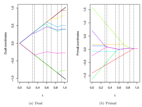
Dual path algorithm

$\hat{\beta}=\operatorname{argmin}{\beta \in \mathbb{R}^{n}}\left{\frac{1}{2}|y-\beta|{2}^{2}+\lambda \sum_{\left(j, j^{\prime}\right) \in E}\left|\beta_{j}-\beta_{j^{\prime}}\right|\right}$

$\hat{u}(\lambda)=\underset{u \in \mathbb{R}^{m}}{\operatorname{argmin}}\left|y-D^{\top} u\right|_{2}^{2} \quad \text { subject to }|u|_{\infty} \leq \lambda$

$\hat{\beta}(\lambda)=y-D^{\top} \hat{u}(\lambda)$

The kth step

The algorithm begins with $λ = ∞$, and then proceeds through a series of steps,corresponding to decreasing values of $λ$.

$\hat{\beta}(\lambda)=P_{\operatorname{Null}\left(D_{-B_{k}}\right)}\left(y-\lambda \cdot D_{B_{k}}^{\top} s_{B_{k}}\right)$

boundary set $B_k ⊆ [m]$,which consists of the subset of indices of the vector $u$ for which the inequality constraint in dual problem is tight.

$s_{B_k} $ , the signs of the elements of $u$ associated with this boundary set, are also computed.

$D_{B_{k}}$ and $D_{-B_{k}}$ correspond to the submatrices of D with rows in $B_{k}$ and not in $B_{k}$ , respectively, and $P_{\operatorname{Null}\left(D_{-B_{k}}\right)}$ is the projection matrix onto the null space of $D_{-B_{k}}$ .

For the generalized lasso, $\hat{\beta}$ can be computed from $\lambda$ and $(B_k, s_{B_k})$ from the dual path algorithm.

$p_{Hyun}$

To control the selective Type I error in the sense of (6), we must condition on the information used to construct that null hypothesis.

To test a null hypothesis of the form $H_0 : ν^Tβ = 0$ where $ν$ is a function of the data, we must condition on the information used to construct $ν$.

$p_{\text {Hyun }} \equiv \mathbb{P}_{H_{0}}\left(\left|\nu^{\top} Y\right| \geq\left|\nu^{\top} y\right| \mid \bigcap_{k=1}^{K}\left{M_{k}(Y)=M_{k}(y)\right}, \Pi_{\nu}^{\perp} Y=\Pi_{\nu}^{\perp} y\right)$

$M_{k}(y) \equiv\left(B_{k}(y), s_{B_{k}}(y), R_{k}(y), L_{k}(y)\right)$

The set of $Y$ that leads to a specified output for the first $K$ steps of the dual path algorithm for generalized lasso is a polyhedron, $i.e. {Y: A Y \leq 0} $, for a matrix $A$ that can be explicitly computed.

The set $ \left{Y \in \mathbb{R}^{n}: \bigcap_{k=1}^{K}\left{M_{k}(Y)=M_{k}(y)\right}\right}$ is of the form ${Y: A Y \leq 0}$ for some matrix A that can be constructed explicitly based on $M_{1}(y), \ldots, M_{K}(y) $.

dual path algorithm for generalized lasso -->a polyhedron $ {Y: A Y \leq 0} $ --> truncated normal distribution --> compute $p_{Hyun}$.

Our method

$p_{\hat{C}_{1}, \hat{C}_{2}}$

The outputs of the first $K-1$ steps of the dual path algorithm are not considered in constructing $ν$.

In fact, the data analyst need only condition on $B_K$ and $s_{B_K}$.

$p_{\hat{C}_{1}, \hat{C}_{2}} \equiv \mathbb{P}_{H_{0}}\left(\left|\nu^{\top} Y\right| \geq\left|\nu^{\top} y\right| \mid \hat{C}_{1}(y), \hat{C}_{2}(y) \in \mathcal{C C}_{K}(Y), \Pi_{\nu}^{\perp} Y=\Pi_{\nu}^{\perp} y\right)$

$\hat{C}{1}(y), \hat{C}{2}(y)$ are two connected components estimated from the data realization $y$ and used to construct the contrast vector $ν$ in (5), and $\mathcal{C C}_{K}(Y)$ is the set of connected components obtained from applying $K$ steps of the dual path algorithm.

Properties of $p_{\hat{C}_{1}, \hat{C}_{2}}$

Suppose that $Y \sim \mathcal{N}\left(\beta, \sigma^{2} I_{n}\right)$. Let $\phi \sim \mathcal{N}\left(0, \sigma^{2}|\nu|_{2}^{2}\right)$.

Define $y^{\prime}(\phi)=\Pi_{\nu}^{\perp} y+\phi \cdot \frac{\nu}{|\nu|_{2}^{2}}=y+\left(\frac{\phi-\nu^{\top} y}{|\nu|_{2}^{2}}\right) \nu$

Then $p_{\hat{C}_{1}, \hat{C}_{2}}=\mathbb{P}\left(|\phi| \geq\left|\nu^{\top} y\right| \mid \hat{C}_{1}(y), \hat{C}_{2}(y) \in \mathcal{C} \mathcal{C}_{K}\left(y^{\prime}(\phi)\right)\right)$

Therefore, to compute the $p_{\hat{C}_{1}, \hat{C}_{2}}$

It suffices to characterize the set $\mathcal{S}{\hat{C}{1}, \hat{C}{2}} \equiv\left{\phi \in \mathbb{R}: \hat{C}{1}(y), \hat{C}{2}(y) \in \mathcal{C C}{K}\left(y^{\prime}(\phi)\right)\right}$
$\mathcal{S}{\hat{C}{1}, \hat{C}_{2}}$can be expressed as a union of intervals, each of which can be computed by applying Corollary 1 on $y^{\prime}(\phi)$ .
Corollary 1: The set $\left{\phi \in \mathbb{R}: \bigcap_{k=1}^{K}\left{M_{k}\left(y^{\prime}(\phi)\right)=M_{k}(y)\right}\right}$ is an interval.
we use Proposition 4 to develop an efficient recipe to compute $ \mathcal{S}{\hat{C}{1}, \hat{C}{2}}$ by constructing the index set $\mathcal{J}$ and scalars $\ldots<a{-2}<a_{-1}<a_{0}<a_{1}<a_{2}<\ldots$ . (P32 Appendix.3)
use $p_{\hat{C}_{1}, \hat{C}_{2}}(\delta)=\mathbb{P}\left(|\phi| \geq\left|\nu^{\top} y\right| \mid \phi \in \tilde{\mathcal{S}}_{\hat{C}_{1}, \hat{C}_{2}}\right)$ for brevity (P37 Appendix.6)

Extension

Confifidence intervals for $\nu^{\top} \beta$

$\mathbb{P}\left(\nu^{\top} \beta \in\left[\theta_{l}\left(\nu^{\top} Y\right), \theta_{u}\left(\nu^{\top} Y\right)\right] \mid \hat{C}_{1}, \hat{C}_{2} \in \mathcal{C} \mathcal{C}_{K}(Y), \Pi_{\nu}^{\perp} Y=\Pi_{\nu}^{\perp} y\right)=1-\alpha$

Define functions $\theta_{l}(t)$ and $\theta_{u}(t)$ such that $F_{\theta_{l}(t), \sigma^{2}|\nu|_{2}^{2}}^{\mathcal{S}_{\hat{C}_{1}, \hat{C}_{2}}}(t)=1-\frac{\alpha}{2}, \quad F_{\theta_{u}(t), \sigma^{2}|\nu|_{2}^{2}}^{\mathcal{S}_{\hat{C}_{1}, \hat{C}_{2}}}(t)=\frac{\alpha}{2}$

where $F_{\mu, \sigma^{2}}^{\mathcal{S}_{\hat{C}_{1}, \hat{C}_{2}}}(t)$ is the cumulative distribution function of a $\mathcal{N}\left(\mu, \sigma^{2}\right)$ random variable, truncated to the set $\mathcal{S}_{\hat{C}_{1}, \hat{C}_{2}} $ . Then $\left[\theta_{l}\left(\nu^{\top} Y\right), \theta_{u}\left(\nu^{\top} Y\right)\right]$ has $(1-\alpha)$ selective coverage.

An alternative conditioning set

$p_{\hat{C}_{1}, \hat{C}_{2}}^{*}=\mathbb{P}_{H_{0}}\left(\left|\nu^{\top} Y\right| \geq\left|\nu^{\top} y\right| \mid \hat{C}_{1}(y), \hat{C}_{2}(y) \in \mathcal{C} \mathcal{C}(Y), \Pi_{\nu}^{\perp} Y=\Pi_{\nu}^{\perp} y\right)$

the function $CC$ now represents the graph fused lasso estimator tuned to yield exactly $L$ connected components.

Simulation

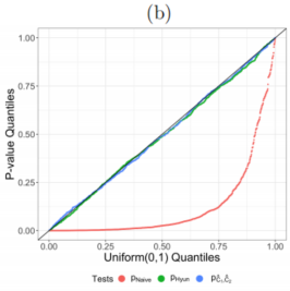
$p_{\text {Naive }} \equiv \mathbb{P}_{H_{0}}\left(\left|\nu^{\top} Y\right| \geq\left|\nu^{\top} y\right|\right)$

One-dimensional fused lasso

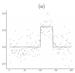
$Y_{j} \stackrel{\text { ind. }}{\sim} \mathcal{N}\left(\beta_{j}, \sigma^{2}\right), \quad \beta_{j}=\delta \times 1_{(101 \leq j \leq 140)}, \quad j=1, \ldots, 200$

Figure $3(a)$ displays an example of this synthetic data with $δ = 3$ and $σ = 1$.

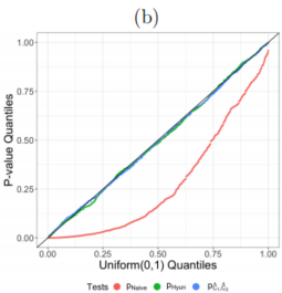
We simulated $y_1, . . . , y_{200}$ with $δ = 0$ and $σ = 1$, and solved (3) with $K = 2$ steps in the dual path algorithm, which yields exactly three estimated connected components by the properties of the one-dimensional fused lasso.

Figure $3(b)$ displays the observed p-value quantiles versus $Uniform(0,1)$ quantiles.

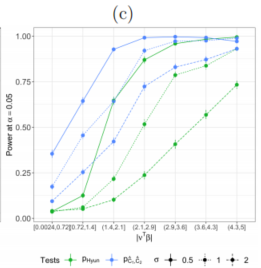
We generated 1,500 datasets from (22) with $σ ∈ {0.5, 1, 2}$, for each of ten evenly-spaced values of $δ ∈ [0.5, 5]$. For every simulated dataset, we solved (3) with $K = 2$. We then rejected : $H_0: \nu^{\top} \beta$ if $p_{\text {Hyun }}$ or $p_{\hat{C}_{1}, \hat{C}_{2}}$ was less than $α = 0.05$.

Two-dimensional fused lasso

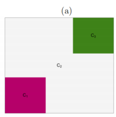
$Y_{j} \stackrel{\text { ind. }}{\sim} \mathcal{N}\left(\beta_{j}, \sigma^{2}\right), \quad \beta_{j}=\delta \times 1_{j \in C_{1}}+(-\delta) \times 1_{j \in C_{3}}, \quad j=1, \ldots, 64$

Figure $4(a)$ displays an example of constant segments with means $δ，0，-\delta$.

We simulated $y_1, . . . , y_{64}$ with $δ = 0$ and $σ = 1$, and solved (3) with $K = 15$ steps in the dual path algorithm, which yields between 2 and 4 estimated connected components.

Figure $4(b)$ displays the observed p-value quantiles versus $Uniform(0,1)$ quantiles.

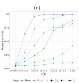
We generated 1,500 datasets from (22) with $σ ∈ {0.5, 1, 2}$, for each of ten evenly-spaced values of $δ ∈ [0.5, 4]$. For every simulated dataset, we solved (3) with $K = 15$. We then rejected : $H_0: \nu^{\top} \beta$ if $p_{\text {Hyun }}$ or $p_{\hat{C}_{1}, \hat{C}_{2}}$ was less than $α = 0.05$.

知识补充：

文献

14 Fithian selective type 1 error;(10)式消除冗余参数
16 Lee: polyhedral
11 Taylor: dual path algorithm